Environment90m layers
We recently prepared a new dataset called Environment90m!
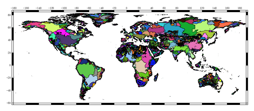
For each of the roughly 726 million sub-catchments present in Hydrography90m, it provides detailed data on soil condition, bioclimatic variables, land cover, and many more. Just like the Hydrography90m layers, it is openly available for download, and easy to download using the dedicated functions in the R package hydrographr.
Here is an overview of all tables in the dataset. It consists of the summary statistics of 112 environmental layers in 7 categories which we calculated for each single sub-catchment of the Hydrography90m dataset (Amatulli et al. (2022), see references below).
Please see the paper by Garcia Marquez et al. (2026) for further details (see references below).
- Land Cover
- Bioclimatic variables
- Soil
- Stream Flow
- Elevation
- Aridity and Evapotranspiration
- Hydrography90m variables
For downloading and working with the data, we recommend using the R package hydrographr. Examples of how to do this are included below. A full vignette showing how to prepare and process the data needed to run a species distribution model to predict the habitat suitability of a fish species in a specific basin can be found at https://glowabio.github.io/hydrographr/articles/case_study_Danube.html.
Please note that the dataset is protected by the Creative Commons Attribution-Non-Commercial 4.0 International License (CC BY-NC 4.0).
If you use our dataset in a publication, please also cite our work as:
- García Márquez, J. R., Grigoropoulou, A., Tomiczek, T., Schürz, M., Bremerich, V., Torres-Cambas, Y., Buurman, M., Amatulli, G., and Domisch, S. (2026): Environment90m - globally standardized environmental variables for freshwater science at high spatial resolution. Earth System Science Data, 18, 1541-1559, doi:10.5194/essd-18-1541-2026.
Citations of the work used to prepare this datasets can be found at the bottom of this page.
Pick a tile!
… to generate download links.
If you click on any tile, the sections below will feature download links and R code for that specific tile!
(No tile selected yet)
Land Cover (ESA-CCI)
For land use data, we aggregated the consistent global land cover maps of the Land Cover European Space Agency (ESA) Climate Change Initiative (CCI) project into 22 categories from the original 37 ESA category level 2 land cover classes at a spatial resolution of 300m (CCI (2017), see references below). The annual data are available for the years 1992 to 2020. The data source is ESA (2017) (see references below).
- How to download the data using the R package hydrographr:
download_landcover_tables(
base_vars=c(“c10”, “c130”), years=c(1992), tile_ids=c(“h00v04”), download_dir=”.”, download=TRUE)
Directory containing all the variables: public.igb-berlin.de
Pick a year to generate download links for all land cover variables for that year:
| c10: Cropland, rainfed |
|---|
| Cropland, rainfed. Combined classes 10+11+12. |
| Unit: Proportion |
Download link for selectedd tile |
| c20: Cropland, irrigated/post-flooding |
| Cropland, irrigated or post-flooding. |
| Unit: Proportion |
Download link for selected tile |
| c30: Cropland/natural vegetation |
| Mosaic cropland (>50%) - natural vegetation (tree, shrub, herbaceous cover) (<50%). |
| Unit: Proportion |
Download link for selected tile |
| c40: Natural vegetation/cropland |
| Mosaic natural vegetation (tree, shrub, herbaceous cover) (>50%) / cropland (<50%). |
| Unit: Proportion |
Download link for selected tile |
| c50: Tree cover, broadleaved, evergreen |
| Tree cover, broadleaved, evergreen, closed to open (>15%). |
| Unit: Proportion |
Download link for selected tile |
| c60: Tree cover, broadleaved, deciduous |
| Tree cover, broadleaved, deciduous, closed to open (>15%). Combined classes: 60+61+62. |
| Unit: Proportion |
Download link for selected tile |
| c70: Tree cover, needleleaved, evergreen |
| Tree cover, needleleaved, evergreen, closed to open (>15%). Combined classes 70+71+72. |
| Unit: Proportion |
Download link for selected tile |
| c80: Tree cover, needleleaved, deciduous |
| Tree cover, needleleaved, deciduous, closed to open (>15%). Combined classes 80+81+82. |
| Unit: Proportion |
Download link for selected tile |
| c90: Tree cover, mixed leaf type |
| Tree cover, mixed leaf type (broadleaved and needleleaved). |
| Unit: Proportion |
Download link for selected tile |
| c100: Tree and shrub |
| Mosaic tree and shrub (>50%) / herbaceous cover (<50%). |
| Unit: Proportion |
Download link for selected tile |
| c110: Herbaceous/tree and shrub |
| Mosaic herbaceous cover (>50%) / tree and shrub (<50%). |
| Unit: Proportion |
Download link for selected tile |
| c120: Shrubland |
| Shrubland. Combined classes 120+121+122. |
| Unit: Proportion |
Download link for selected tile |
| c130: Grassland |
| Grassland. |
| Unit: Proportion |
Download link for selected tile |
| c140: Lichens, mosses |
| Lichens, mosses. |
| Unit: Proportion |
Download link for selected tile |
| c150: Sparse vegetation |
| Sparse vegetation (tree, shrub, herbaceous cover) (<15%). Combined classes 150+151+152+153. |
| Unit: Proportion |
Download link for selected tile |
| c160: Tree cover, flooded, fresh/brackish water |
| Tree cover, flooded, fresh or brackish water. |
| Unit: Proportion |
Download link for selected tile |
| c170: Tree cover, flooded, saline water |
| Tree cover, flooded, saline water. |
| Unit: Proportion |
Download link for selected tile |
| c180: Shrub or herbaceous |
| Shrub or herbaceous cover, flooded, fresh - saline - brackish water. |
| Unit: Proportion |
Download link for selected tile |
| c190: Urban areas |
| Urban areas. |
| Unit: Proportion |
Download link for selected tile |
| c200: Bare areas |
| Bare areas. Combined classes 200+201+202. |
| Unit: Proportion |
Download link for selected tile |
| c210: Water bodies |
| Water bodies. |
| Unit: Proportion |
Download link for selected tile |
| c220: Snow and ice |
| Permanent snow and ice. |
| Unit: Proportion |
Download link for selected tile |
Bioclimatic Variables (CHELSA)
We derived high-resolution climate information from the Chelsa v2.1 dataset available at chelsa-climate.org (Karger et al. 2017, 2021, see references below). We used 19 bioclimatic variables (bio 1 to 19) at 30-arc-sec (ca. 1 km²) resolution for 30-year averages of temperature and precipitation. We aggregated the data for three time ranges: from 1981 to 2010, corresponding to observational data, and future projections for the years 2041 to 2070, as well as 2071 to 2100, corresponding to 2050 and 2070, respectively. For each future projection, we used general circulation models (GCMs) following three shared socioeconomic pathways (SSP1-RCP2.6, SSP3-RCP7, and SSP5-RCP8.5; Ebi et al. (2014); O’Neill et al. (2017), see references below).
- How to download observed data using the R package hydrographr:
download_observed_climate_tables(
subset = c(“bio01_1981-2010_observed”), tile_ids = c(“h00v04”), download = TRUE, download_dir = “.”)
- How to download projected data using the R package hydrographr:
download_projected_climate_tables(
subset = c(“bio01_2071-2100_ukesm1-0-ll_ssp585_v2_1”), tile_ids = c(“h00v04”), download_dir = “.”, download = TRUE)
You can also specify the separate aspects separately (time period, scenario, …):
download_projected_climate_tables(
base_vars = c(“bio01”), time_periods = c(“2071-2100”), models=c(“ukesm1-0-ll”), scenarios=c(“ssp585”), version=c(“v2_1”), tile_ids = c(“h00v04”), download = TRUE)
Directory containing all the variables: public.igb-berlin.de
Pick a time period to generate download links for all bioclim variables for that period:
- Pick a model to generate download links for all bioclim variables for that model:
- Pick a scenario to generate download links for all bioclim variables for that scenario:
| bio01: Annual mean temperature |
|---|
| Mean annual daily mean air temperatures averaged over 1 year. |
| Unit: Degrees Celsius Scale: 0.1 Offset: -273.15 |
Download link for selected tile |
| bio02: Mean diurnal range |
| Mean diurnal range of temperatures averaged over 1 year. |
| Unit: Degrees Celsius Scale: 0.1 Offset: - |
Download link for selected tile |
| bio03: Isothermality |
| Ratio of diurnal variation to annual variation in temperatures. |
| Unit: Degrees Celsius Scale: 0.1 Offset: - |
Download link for selected tile |
| bio04: Temperature seasonality |
| Standard deviation of the monthly mean temperatures. |
| Unit: Degrees Celsius / 100 Scale: 0.1 Offset: None. |
Download link for selected tile |
| bio05: Max temperature of warmest month |
| The highest temperature of any monthly daily mean maximum temperature. |
| Unit: Degrees Celsius Scale: 0.1 Offset: -273.15 |
Download link for selected tile |
| bio06: Min temperature of coldest month |
| The lowest temperature of any monthly daily mean minimum temperature. |
| Unit: Degrees Celsius Scale: 0.1 Offset: -273.15 |
Download link for selected tile |
| bio07: Temperature annual range |
| The difference between the Maximum Temperature of Warmest month and the Minimum Temperature of Coldest month. |
| Unit: Degrees Celsius Scale: 0.1 Offset: - |
Download link for selected tile |
| bio08: Mean temperature of wettest quarter |
| The wettest quarter of the year is determined (to the nearest month). |
| Unit: Degrees Celsius Scale: 0.1 Offset: -273.15 |
Download link for selected tile |
| bio09: Mean temperature of driest quarter |
| The driest quarter of the year is determined (to the nearest month). |
| Unit: Degrees Celsius Scale: 0.1 Offset: -273.15 |
Download link for selected tile |
| bio10: Mean temperature of warmest quarter |
| The warmest quarter of the year is determined (to the nearest month). |
| Unit: Degrees Celsius Scale: 0.1 Offset: -273.15 |
Download link for selected tile |
| bio11: Mean temperature of coldest quarter |
| The coldest quarter of the year is determined (to the nearest month). |
| Unit: Degrees Celsius Scale: 0.1 Offset: -273.15 |
Download link for selected tile |
| bio12: Annual precipitation |
| Accumulated precipitation amount over 1 year. |
| Unit: kg/m² Scale: 0.1 Offset: - |
Download link for selected tile |
| bio13: Precipitation of wettest month |
| The precipitation amount of the wettest month. |
| Unit: kg/m² Scale: 0.1 Offset: - |
Download link for selected tile |
| bio14: Precipitation of driest month |
| The precipitation amount of the driest month. |
| Unit: kg/m² Scale: 0.1 Offset: - |
Download link for selected tile |
| bio15: Precipitation seasonality |
| The Coefficient of Variation is the standard deviation of the monthly precipitation estimates expressed as a percentage of the mean of those estimates (i.e. the annual mean). |
| Unit: kg/m² Scale: 0.1 Offset: - |
Download link for selected tile |
| bio16: Precipitation of wettest quarter |
| The wettest quarter of the year is determined (to the nearest month). |
| Unit: kg/m² Scale: 0.1 Offset: - |
Download link for selected tile |
| bio17: Precipitation of driest quarter |
| The driest quarter of the year is determined (to the nearest month). |
| Unit: kg/m² Scale: 0.1 Offset: - |
Download link for selected tile |
| bio18: Precipitation of warmest quarter |
| The warmest quarter of the year is determined (to the nearest month). |
| Unit: kg/m² Scale: 0.1 Offset: - |
Download link for selected tile |
| bio19: Precipitation of coldest quarter |
| The coldest quarter of the year is determined (to the nearest month). |
| Unit: kg/m² Scale: 0.1 Offset: - |
Download link for selected tile |
Soil (SoilGrids250)
The soil dataset consists of 16 variables that represent chemical and physical soil properties globally. These variables were sourced from the global gridded soil information dataset, SoilGrids250 v2.0, which is originally provided at seven standard depths for each numerical soil property (with the exception of depth to bedrock and soil organic carbon content) and at a spatial resolution of 250 m (Hengl et al. (2017), see references below). To integrate all soil depths (up to 220 cm), we calculated the weighted average for each soil property originally measured at different depths (Hengl et al. (2017)) and finally aggregated the 16 variables across Hydrography90m sub-catchments (Amatulli et al. (2022), see references below).
- How to download the data using the R package hydrographr:
download_soil_tables(
subset = c(“clyppt”), tile_ids = c(“h00v04”), download_dir = “.”, download = TRUE)
- Directory containing all the variables: public.igb-berlin.de
| awcts: Derived saturated water content |
|---|
| Derived saturated water content. |
| Unit: - |
Download link for selected tile |
| clyppt: Clay content |
| Clay content. |
| Unit: Percent |
Download link for selected tile |
| sndppt: Sand content |
| Sand content. |
| Unit: Percent |
Download link for selected tile |
| sltppt: Silt content |
| Silt content. |
| Unit: Percent |
Download link for selected tile |
| wwp: Derived available soil water capacity |
| Derived available soil water capacity. |
| Unit: - |
Download link for selected tile |
| texmht: Texture class |
| Texture class. Following the USDA classification. |
| Unit: - |
Download link for selected tile |
| orcdrc: Soil organic carbon content |
| Soil organic carbon content. |
| Unit: g/kg. |
Download link for selected tile |
| phihox: Soil pH |
| Soil pH x 10 in H2O. |
| Unit: pH |
Download link for selected tile |
| bldfie: Bulk density |
| Bulk density. |
| Unit: Kg/m³ |
Download link for selected tile |
| cecsol: Cation exchange capacity |
| Cation exchange capacity. |
| Unit: cmolc/kg |
Download link for selected tile |
| crfvol: Coarse fragments volumetric |
| Coarse fragments volumetric. |
| Unit: Percent |
Download link for selected tile |
| acdwrb: Grade of a sub-soil being acid |
| Grade of a sub-soil being acid, e.g. having a pH < 5 and low BS. |
| Unit: pH. |
Download link for selected tile |
| bdricm: Depth to bedrock |
| Depth to bedrock (r horizon) up to 200 cm. |
| Unit: cm |
Download link for selected tile |
| bdrlog: Probability of occurence of r horizon |
| Probability of occurence of e horizon. |
| Unit: Percent |
Download link for selected tile |
| histpr: Cumulative probability of organic soil |
| Cumulative probability of organic soil based on the TAXOUSDA and TAXNWRB. |
| Unit: -. |
Download link for selected tile |
| slgwrb: Sodic soil grade |
| Sodic soil grade based on WRB soil types and soil pH. |
| Unit: pH |
Download link for selected tile |
Stream Flow (FLO1K)
For stream flow we used the FLO1K dataset which comprises the mean, maximum and minimum annual flow for each year in the period 1960–2015, provided as spatially continuous gridded layers at a high spatial resolution of 30 arc-seconds (ca. 1 km²) (Barbarossa et al. (2018), see references below). From this dataset, we only used the data from 1980 - 2010 and averaged it across this time to match the CHELSA observed climate dataset (see above).
- How to download the data using the R package hydrographr:
download_flo1k_tables(
subset = c(“flo1k”), tile_ids = c(“h00v04”), download_dir = “.”, download = TRUE)
- Directory containing all the variables: public.igb-berlin.de
| flo1k: Stream flow |
|---|
| The long-term mean annual flow represents the average of the year-specific FLO1K maps for mean Annual Flow over the period 1980 - 2010. |
| Unit: m³/s. Scale: - Offset: - |
Download link for selected tile |
Elevation (MERIT-DEM)
To represent the elevation variable we used the 90 m resolution Multi-Error-Removed Improved-Terrain Digital Elevation Model (MERIT DEM) v1.0.3 (Yamazaki et al. (2017), see references below). The error removal procedures have improved the vertical accuracy of this product.
Spatial Resolution: 90m²
- How to download the data using the R package hydrographr:
download_merit_dem_tables(
subset = c(“elev”), tile_ids = c(“h00v04”), download_dir = “.”, download = TRUE)
- Directory containing all the variables: public.igb-berlin.de
| elev: Mean elevation |
|---|
| The MERIT DEM represents elevation in meters (mean elevation of the sub-catchment). |
| Unit: m |
Download link for selected tile |
Aridity and Evapotranspiration (cgiar csi v.3)
This dataset provides global raster data on evapotranspiration processes and rainfall deficit for potential vegetation growth, at a high spatial resolution of 30 arc-seconds (ca. 1 km²). Global Aridity and Potential Evapotranspiration are both modeled using data available from WorldClim Global Climate Data. The data is available for the 1970 - 2000 period (Zomer and Trabucco (2022), see references below).
- How to download the data using the R package hydrographr:
download_cgiar_tables(
subset = c(“garid”), tile_ids = c(“h00v04”), download_dir = “.”, download = TRUE)
- Directory containing all the variables: public.igb-berlin.de
| gevapt: Evapotranspiration |
|---|
| Potential Evapo-Transpiration (ET0) based upon implementation of the FAO-56 Penman-Monteith Reference Evapotranspiration (ET0) equation. |
| Unit: mm Scale: - Offset: - |
Download link for selected tile |
| garid: Aridity Index |
| Ratio between precipitation and ET0. Values reported have been multiplied by a factor of 10.000 |
| Unit: - Scale: - Offset: (Values reported have been multiplied by a factor of 10.000) |
Download link for selected tile |
Hydrography90m
The Hydrography90m is a high-resolution (∼90 m) dataset delineating a global stream channel network (Amatulli et al. (2022), see references below) and serves as the base of Environment90m. The calculation of Hydrography90m used the MERIT Hydro Digital Elevation Model at 3 arcsec (∼90 m at the Equator) (Yamazaki et al. (2017), see references below). The main feature of Hydrography90m is the delineation of small headwater streams. In addition, this dataset includes a number of stream topographic and topological properties. The summary statistics of the Environment90m dataset presented here are calculated for each of the 726 million unique sub-catchments of the Hydrography90m, which also serve as the spatial units in Environment90m.
- How to download the data using the R package hydrographr:
download_hydrography90m_tables(
subset = c(“cti”), tile_ids = c(“h00v04”), download_dir = “.”, download = TRUE)
- How to download the same variables as spatial data (GeoTIFF and/or geopackage files), using the function download_tiles:
download_tiles(
variable = “cti”, file_format = “tif”, tile_id = c(“h00v04”), download_dir = “.”)
- Directory containing all the variables: public.igb-berlin.de
For detailed explanations of the variables, please refer to the neighbour page hydrography90m_layers:
- accumulation (download link for selected tile)
- slope_curv_max_dw_cel (download link for selected tile)
- slope_curv_min_dw_cel (download link for selected tile)
- slope_elv_dw_cel (download link for selected tile)
- slope_grad_dw_cel (download link for selected tile)
- stream_dist_dw_near (download link for selected tile)
- stream_dist_proximity (download link for selected tile)
- stream_dist_up_farth (download link for selected tile)
- stream_dist_up_near (download link for selected tile)
- outlet_dist_dw_basin (download link for selected tile)
- outlet_dist_dw_scatch (download link for selected tile)
- stream_diff_dw_near (download link for selected tile)
- stream_diff_up_farth (download link for selected tile)
- stream_diff_up_near (download link for selected tile)
- outlet_diff_dw_basin (download link for selected tile)
- outlet_diff_dw_scatch (download link for selected tile)
- channel_curv_cel (download link for selected tile)
- channel_dist_dw_seg (download link for selected tile)
- channel_dist_up_cel (download link for selected tile)
- channel_dist_up_seg (download link for selected tile)
- channel_elv_dw_cel (download link for selected tile)
- channel_elv_dw_seg (download link for selected tile)
- channel_elv_up_cel (download link for selected tile)
- channel_elv_up_seg (download link for selected tile)
- channel_grad_dw_seg (download link for selected tile)
- channel_grad_up_cel (download link for selected tile)
- channel_grad_up_seg (download link for selected tile)
- order_hack (download link for selected tile)
- order_horton (download link for selected tile)
- order_shreve (download link for selected tile)
- order_strahler (download link for selected tile)
- order_topo (download link for selected tile)
- cti (download link for selected tile)
- spi (download link for selected tile)
- sti (download link for selected tile)
Some variables are not included in Hydrography90m, so we explain them here:
10 stream reach layers:
- length: Length of the stream reach (download link for selected tile)
- stright: Straight length / Length of the stream as straight line (download link for selected tile)
- sinosoid: Sinusoid of the stream reach / Fractal dimension: Stream length/straight stream length (download link for selected tile)
- cum_length: Accumulated length / Length of stream from source (download link for selected tile)
- out_dist: Distance to outlet / Distance of current stream init from outlet (download link for selected tile)
- source_elev: Source elevation / Elevation of stream init (download link for selected tile)
- outlet_elev: Outlet elevation / Elevation of stream outlet (download link for selected tile)
- elev_drop: Elevation drop / Difference between source_elev and outlet_elev + drop outlet (download link for selected tile)
- out_drop: Outlet drop / Drop at the outlet of the stream (download link for selected tile)
- gradient: Gradient / Mean gradient of the sub-catchment (downstream elevation difference divided by distance) (download link for selected tile)
1 stream connectivity layer:
- connections: TODO add description (download link for selected tile)
References
Environment90m:
- García Márquez, J. R., Grigoropoulou, A., Tomiczek, T., Schürz, M., Bremerich, V., Torres-Cambas, Y., Buurman, M., Amatulli, G., and Domisch, S.: Environment90m - globally standardized environmental variables for freshwater science at high spatial resolution. Earth System Science Data, 18, 1541-1559, doi:10.5194/essd-18-1541-2026, 2026.
Hydrography90m:
- Amatulli, G., Garcia Marquez, J.R., Sethi, T., Kiesel, J., Grigoropoulou, A., Üblacker, M., Shen, L., Domisch, S.: Hydrography90m: A new high-resolution global hydrographic dataset. Earth System Science Data, 14, 4525–4550, doi:10.5194/essd-14-4525-2022, 2022.
Bioclimatic variables:
- Karger, D. N., Conrad, O., Böhner, J., Kawohl, T., Kreft, H., Soria-Auza, R. W., Zimmermann, N. E., Linder, H. P., and Kessler, M.: Climatologies at high resolution for the earth’s land surface areas, Scientific data, 4, 1–20, 2017.
- Karger, D. N., Conrad, O., Böhner, J., Kawohl, T., Kreft, H., Soria-Auza, R. W., Zimmermann, N. E., Linder, H. P., and Kessler, M.: Climatologies at high resolution for the earth’s land surface areas, Scientific Data, 4, 170 122, doi:10.1038/sdata.2017.122, 2017.
- Karger, D. N., Conrad, O., Böhner, J., Kawohl, T., Kreft, H., Soria-Auza, R. W., Zimmermann, N. E., Linder, H. P., and Kessler, M.: Climatologies at high resolution for the earth’s land surface areas, doi:10.16904/envidat.228, 2021.
- Ebi, K. L., Hallegatte, S., Kram, T., Arnell, N. W., Carter, T. R., Edmonds, J., Kriegler, E., Mathur, R., O’Neill, B. C., Riahi, K., et al.: A new scenario framework for climate change research: background, process, and future directions, Climatic Change, 122, 363–372, 2014.
- O’Neill, B. C., Kriegler, E., Ebi, K. L., Kemp-Benedict, E., Riahi, K., Rothman, D. S., Van Ruijven, B. J., Van Vuuren, D. P., Birkmann, J., Kok, K., et al.: The roads ahead: Narratives for shared socioeconomic pathways describing world futures in the 21st century, Global environmental change, 42, 169–180, 2017.
Soil:
- Hengl, T., Mendes de Jesus, J., Heuvelink, G. B. M., Ruiperez Gonzalez, M., Kilibarda, M., Blagotić, A., Shangguan, W., Wright, M. N., Geng, X., Bauer-Marschallinger, B., Guevara, M. A., Vargas, R., MacMillan, R. A., Batjes, N. H., Leenaars, J. G. B., Ribeiro, E., Wheeler, I., Mantel, S., and Kempen, B.: SoilGrids250m: Global gridded soil information based on machine learning, PLOS ONE, 12, e0169 748, doi:10.1371/journal.pone.0169748, 2017.
Land Cover:
- ESA: Land Cover CCI Product User Guide Version 2. Tech. Rep. Available at: maps.elie.ucl.ac.be/CCI/viewer/download/ESACCI-LC-Ph2-PUGv2_2.0.pdf, Tech. rep., European Space Agency, 2017.
- CCI, E. L. C.: Product user guide version 2.0, UCL-Geomatics: London, UK, 685, 2017.
Aridity and Evapotranspiration:
- Zomer, R. J. and Trabucco, A.: Version 3 of the “Global Aridity Index and Potential Evapotranspiration (ET0) Database”: Estimation of Penman-Monteith Reference Evapotranspiration. Available online from the CGIAR-CSI GeoPortal at: https://cgiarcsi.community/2019/0124/global-aridity-index-and-potential-evapotranspiration-climate-database-v3/, Tech. rep., CGIAR-320 CSI, https://cgiarcsi.community/2019/01/24/global-aridity-index-and-potential-evapotranspiration-climate-database-v3, 2022.
Stream flow:
- Barbarossa, V., Huijbregts, M. A. J., Beusen, A. H. W., Beck, H. E., King, H., and Schipper, A. M.: FLO1K, global maps of mean, maximum and minimum annual streamflow at 1 km resolution from 1960 through 2015, Scientific Data, 5, 180 052, doi:10.1038/sdata.2018.52, 2018.
Elevation
- Yamazaki, D., Ikeshima, D., Tawatari, R., Yamaguchi, T., O’Loughlin, F., Neal, J. C., Sampson, C. C., Kanae, S., and Bates, P. D.: A high-accuracy map of global terrain elevations: Accurate Global Terrain Elevation map, Geophysical Research Letters, 44, 5844–5853, doi:10.1002/2017GL072874, 2017.